Intro to Data Science
In this blog post, we will take a bird eye view of various steps involved in a Data Science project, we’ll get from Exploraratory Data Analysis to training a Machine Learning model, if you’re starting with data science, you’ll find this post really helpful !!
so, What is Data Science ?
In a nutshell Data Science has to do with analysis of data through modelling and conducting experiments. Two main problems, for which we use Data Science are inference and prediction.
Inference is a class of problems where we try to find relationships between features using statistical tools and use modelling for understanding the dependence of features on one another.
Prediction, on the other hand is a class of problems where we want to build the most accurate model possible using the data in hand.
Based on the type of problem we are trying to solve, we need to put in place different strategies and use different tools.
Data Science uses alot of statisticals tools, still it is different than statistics, in some sense, due to its ability to work on qualitative data (e.g. images and text) as well. After the advent of Information age, while digital data is omnipresent now, data science seems to have the capability to solve problems which were not possible earlier.
“Data science has become a fourth approach to scientific discovery, in addition to experimentation, modeling, and computation,” said Provost Martha Pollack
Data
The Data contains scores of countries based on parameters like, Gross Development Product or GDP, Freedom, Happiness, Corruption and Life Expectancy. Using these parameters a rating created for every country, Happiness Score this rating defines how much the conditions differ for people living in different countries. Data is collected for 4 years, each corresponding to year from 2015 to 2018, new parameters have been added to recent year’s data
Problem
-
Does Corruption affects Happinesss ?
-
What is happiness score in case of poor countries (Low GDP) ?
-
What makes a Country more happy, Economy (GDP) or Freedom ?
-
What relates most to Happiness ?
Lets write some Code now !!
You can download the jupyter notebook here.
#Importing libraries
import pandas as pd
import numpy as np
import matplotlib.pyplot as plt
import seaborn as  sns
#Reading Files
df_2015 = pd.read_csv('./894_813759_bundle_archive/2015.csv')
df_2016 = pd.read_csv('./894_813759_bundle_archive/2016.csv')

df_2017 = pd.read_csv('./894_813759_bundle_archive/2017.csv')
df_2018 = pd.read_csv('./894_813759_bundle_archive/2018.csv')
#Lets take a look at columns
df_2015.columns,df_2015.shape
(Index(['Country', 'Happiness Rank', 'Happiness Score',
        'Economy (GDP per Capita)', 'Family', 'Health (Life Expectancy)',
        'Freedom', 'Trust (Government Corruption)', 'Generosity'],
       dtype='object'),
 (158, 9))
df_2018.columns,df_2018.shape
(Index(['Overall rank', 'Country or region', 'Score', 'GDP per capita',
        'Social support', 'Healthy life expectancy',
        'Freedom to make life choices', 'Generosity',
        'Perceptions of corruption'],
       dtype='object'),
 (156, 9))
Data Cleaning
As we can see there is some inconsistency in columns between individual daaframes, we need to ensure that same features are used while concatenating them.
df_2015.head()
| Country | Region | Happiness Rank | Happiness Score | Standard Error | Economy (GDP per Capita) | Family | Health (Life Expectancy) | Freedom | Trust (Government Corruption) | Generosity | Dystopia Residual | |
|---|---|---|---|---|---|---|---|---|---|---|---|---|
| 0 | Switzerland | Western Europe | 1 | 7.587 | 0.03411 | 1.39651 | 1.34951 | 0.94143 | 0.66557 | 0.41978 | 0.29678 | 2.51738 |
| 1 | Iceland | Western Europe | 2 | 7.561 | 0.04884 | 1.30232 | 1.40223 | 0.94784 | 0.62877 | 0.14145 | 0.43630 | 2.70201 |
| 2 | Denmark | Western Europe | 3 | 7.527 | 0.03328 | 1.32548 | 1.36058 | 0.87464 | 0.64938 | 0.48357 | 0.34139 | 2.49204 |
| 3 | Norway | Western Europe | 4 | 7.522 | 0.03880 | 1.45900 | 1.33095 | 0.88521 | 0.66973 | 0.36503 | 0.34699 | 2.46531 |
| 4 | Canada | North America | 5 | 7.427 | 0.03553 | 1.32629 | 1.32261 | 0.90563 | 0.63297 | 0.32957 | 0.45811 | 2.45176 |
df_2016.head()
| Country | Region | Happiness Rank | Happiness Score | Lower Confidence Interval | Upper Confidence Interval | Economy (GDP per Capita) | Family | Health (Life Expectancy) | Freedom | Trust (Government Corruption) | Generosity | Dystopia Residual | |
|---|---|---|---|---|---|---|---|---|---|---|---|---|---|
| 0 | Denmark | Western Europe | 1 | 7.526 | 7.460 | 7.592 | 1.44178 | 1.16374 | 0.79504 | 0.57941 | 0.44453 | 0.36171 | 2.73939 |
| 1 | Switzerland | Western Europe | 2 | 7.509 | 7.428 | 7.590 | 1.52733 | 1.14524 | 0.86303 | 0.58557 | 0.41203 | 0.28083 | 2.69463 |
| 2 | Iceland | Western Europe | 3 | 7.501 | 7.333 | 7.669 | 1.42666 | 1.18326 | 0.86733 | 0.56624 | 0.14975 | 0.47678 | 2.83137 |
| 3 | Norway | Western Europe | 4 | 7.498 | 7.421 | 7.575 | 1.57744 | 1.12690 | 0.79579 | 0.59609 | 0.35776 | 0.37895 | 2.66465 |
| 4 | Finland | Western Europe | 5 | 7.413 | 7.351 | 7.475 | 1.40598 | 1.13464 | 0.81091 | 0.57104 | 0.41004 | 0.25492 | 2.82596 |
df_2017.head()
| Country | Happiness.Rank | Happiness.Score | Whisker.high | Whisker.low | Economy..GDP.per.Capita. | Family | Health..Life.Expectancy. | Freedom | Generosity | Trust..Government.Corruption. | Dystopia.Residual | |
|---|---|---|---|---|---|---|---|---|---|---|---|---|
| 0 | Norway | 1 | 7.537 | 7.594445 | 7.479556 | 1.616463 | 1.533524 | 0.796667 | 0.635423 | 0.362012 | 0.315964 | 2.277027 |
| 1 | Denmark | 2 | 7.522 | 7.581728 | 7.462272 | 1.482383 | 1.551122 | 0.792566 | 0.626007 | 0.355280 | 0.400770 | 2.313707 |
| 2 | Iceland | 3 | 7.504 | 7.622030 | 7.385970 | 1.480633 | 1.610574 | 0.833552 | 0.627163 | 0.475540 | 0.153527 | 2.322715 |
| 3 | Switzerland | 4 | 7.494 | 7.561772 | 7.426227 | 1.564980 | 1.516912 | 0.858131 | 0.620071 | 0.290549 | 0.367007 | 2.276716 |
| 4 | Finland | 5 | 7.469 | 7.527542 | 7.410458 | 1.443572 | 1.540247 | 0.809158 | 0.617951 | 0.245483 | 0.382612 | 2.430182 |
df_2018.head()
| Overall rank | Country or region | Score | GDP per capita | Social support | Healthy life expectancy | Freedom to make life choices | Generosity | Perceptions of corruption | |
|---|---|---|---|---|---|---|---|---|---|
| 0 | 1 | Finland | 7.632 | 1.305 | 1.592 | 0.874 | 0.681 | 0.202 | 0.393 |
| 1 | 2 | Norway | 7.594 | 1.456 | 1.582 | 0.861 | 0.686 | 0.286 | 0.340 |
| 2 | 3 | Denmark | 7.555 | 1.351 | 1.590 | 0.868 | 0.683 | 0.284 | 0.408 |
| 3 | 4 | Iceland | 7.495 | 1.343 | 1.644 | 0.914 | 0.677 | 0.353 | 0.138 |
| 4 | 5 | Switzerland | 7.487 | 1.420 | 1.549 | 0.927 | 0.660 | 0.256 | 0.357 |
We will take columns in df_2015 as baseline, as we can see df_2016 is having few extra columns, so we will remove them.
df_2016.drop(['Lower Confidence Interval','Upper Confidence Interval','Region','Dystopia Residual'],axis=1,inplace=True)
df_2015.drop(['Standard Error','Region','Dystopia Residual'],axis=1,inplace=True)
Lets clean rest of dataframes.
df_2015.columns
Index(['Country', 'Happiness Rank', 'Happiness Score',
       'Economy (GDP per Capita)', 'Family', 'Health (Life Expectancy)',
       'Freedom', 'Trust (Government Corruption)', 'Generosity'],
      dtype='object')
df_2017.head()
| Country | Happiness.Rank | Happiness.Score | Whisker.high | Whisker.low | Economy..GDP.per.Capita. | Family | Health..Life.Expectancy. | Freedom | Generosity | Trust..Government.Corruption. | Dystopia.Residual | |
|---|---|---|---|---|---|---|---|---|---|---|---|---|
| 0 | Norway | 1 | 7.537 | 7.594445 | 7.479556 | 1.616463 | 1.533524 | 0.796667 | 0.635423 | 0.362012 | 0.315964 | 2.277027 |
| 1 | Denmark | 2 | 7.522 | 7.581728 | 7.462272 | 1.482383 | 1.551122 | 0.792566 | 0.626007 | 0.355280 | 0.400770 | 2.313707 |
| 2 | Iceland | 3 | 7.504 | 7.622030 | 7.385970 | 1.480633 | 1.610574 | 0.833552 | 0.627163 | 0.475540 | 0.153527 | 2.322715 |
| 3 | Switzerland | 4 | 7.494 | 7.561772 | 7.426227 | 1.564980 | 1.516912 | 0.858131 | 0.620071 | 0.290549 | 0.367007 | 2.276716 |
| 4 | Finland | 5 | 7.469 | 7.527542 | 7.410458 | 1.443572 | 1.540247 | 0.809158 | 0.617951 | 0.245483 | 0.382612 | 2.430182 |
updated_columns = [i.replace('.',' ') for i in df_2017.columns.tolist()]

df_2017.columns = updated_columns
df_2017.drop([ 'Whisker high','Whisker low','Dystopia Residual'],axis=1,inplace = True)
df_2017.rename(columns={'Economy  GDP per Capita ':'Economy (GDP per Capita)',
                   'Health  Life Expectancy ':'Health (Life Expectancy)',
                  'Trust  Government Corruption ':'Trust (Government Corruption)'},inplace=True)
df_2018.rename(columns={'Country or region':'Country',
                        'Score':'Happiness Score',
                   'Overall rank':'Happiness Rank',
                        'GDP per capita':'Economy (GDP per Capita)',
                        'Freedom to make life choices':'Freedom',
                   'Healthy life expectancy':'Health (Life Expectancy)',
                        'Social support':'Family',
                  'Perceptions of corruption':'Trust (Government Corruption)'},inplace=True)
df = pd.concat([df_2015,df_2016,df_2017,df_2018],axis=0).reset_index(drop=True)
We have successfully cleaned our data, now lets do some Data Science !!
Exploratory Data Analysis
Here we will take a quick look into data, by examining distributions followed by the features and checking for missing values.
df.describe()
| Happiness Rank | Happiness Score | Economy (GDP per Capita) | Family | Health (Life Expectancy) | Freedom | Trust (Government Corruption) | Generosity | |
|---|---|---|---|---|---|---|---|---|
| count | 626.000000 | 626.000000 | 626.000000 | 626.000000 | 626.000000 | 626.000000 | 625.000000 | 626.000000 |
| mean | 78.747604 | 5.372021 | 0.918764 | 1.045891 | 0.584299 | 0.415706 | 0.129138 | 0.226981 |
| std | 45.219609 | 1.131774 | 0.409808 | 0.328946 | 0.241948 | 0.154943 | 0.108202 | 0.126854 |
| min | 1.000000 | 2.693000 | 0.000000 | 0.000000 | 0.000000 | 0.000000 | 0.000000 | 0.000000 |
| 25% | 40.000000 | 4.497750 | 0.606755 | 0.847945 | 0.404142 | 0.310500 | 0.056565 | 0.137263 |
| 50% | 79.000000 | 5.307000 | 0.983705 | 1.081274 | 0.632553 | 0.434635 | 0.094000 | 0.208581 |
| 75% | 118.000000 | 6.187250 | 1.239502 | 1.283387 | 0.772957 | 0.538998 | 0.161570 | 0.290915 |
| max | 158.000000 | 7.632000 | 2.096000 | 1.644000 | 1.030000 | 0.724000 | 0.551910 | 0.838075 |
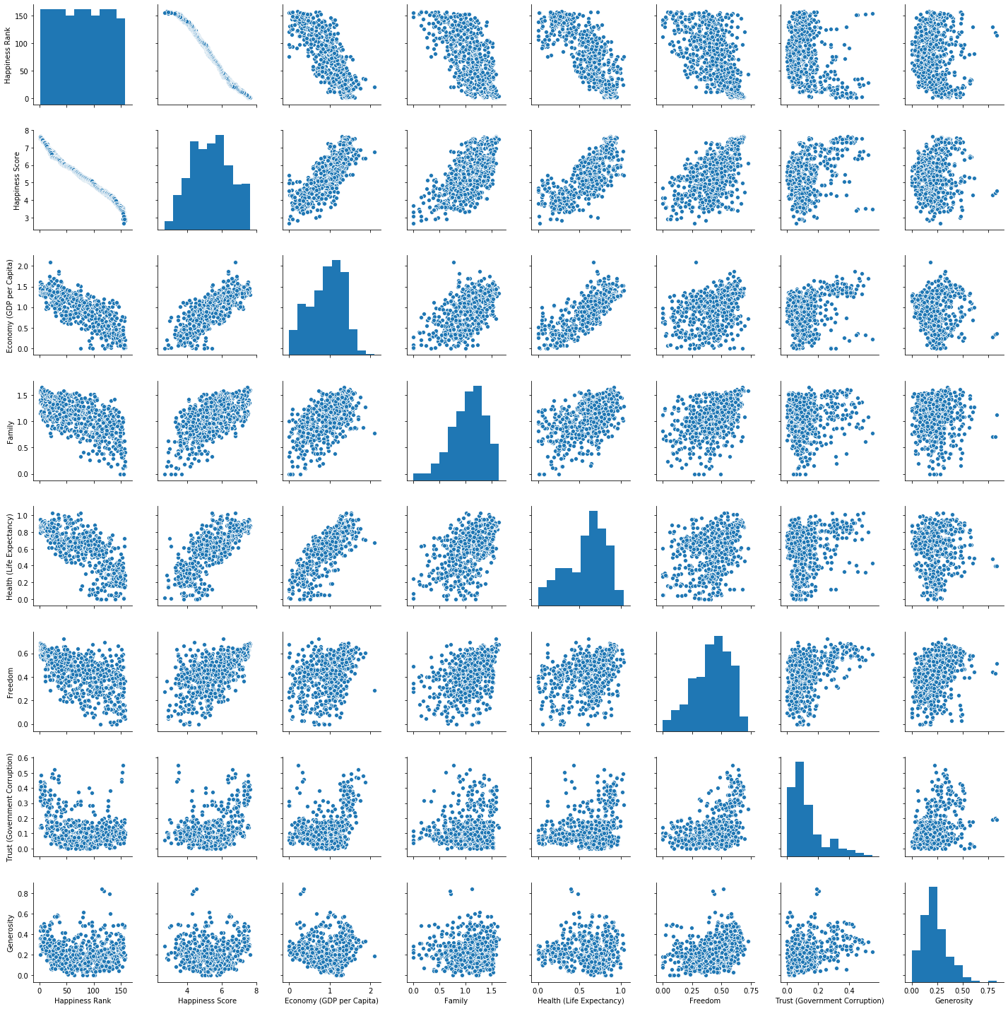
sns.pairplot(df);
Questions we will answer:
-
Does Corruption affects Happinesss ?
-
What makes a Country more happy, Economy (GDP) or Freedom ?
-
What is happiness score in case of poor countries (Low GDP) ?
-
What relates most to Happiness ?
Does Corruption affects Happinesss ?
x = 'Trust (Government Corruption)'
y = 'Happiness Score'
sns.jointplot(data=df,x=x,y=y, kind='reg');
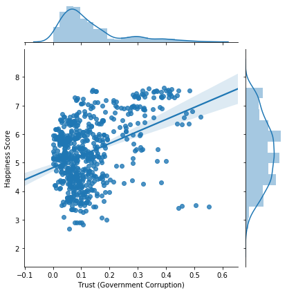
No, Corruption and Happiness are not strongly correlated
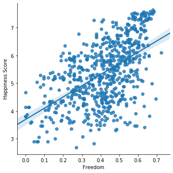
So, What makes a Country more happy ?
x = 'Freedom'
y = 'Happiness Score'
sns.lmplot(data=df,x=x,y=y);
x = 'Economy (GDP per Capita)'
y = 'Happiness Score'
sns.lmplot(data=df,x=x,y=y);
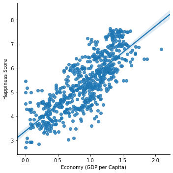
As visible in above graphs, it is clear that Economy of a country has stronger correlation with Happiness than Freedom.
Notes:
- Freedom still has some weak correlation with Happiness
What is happiness score in case of poor countries (Low GDP) ?
We’ll consider the countries having gdp score less than mean (~0.9) as poor.
df_poor = df[df['Economy (GDP per Capita)'] < df['Economy (GDP per Capita)'].mean()]

#filter rich countries
df_rich = df[~(df['Economy (GDP per Capita)'] < df['Economy (GDP per Capita)'].mean())]
df_poor['Happiness Score'].mean()
4.551802119851534
df_rich['Happiness Score'].mean()
6.04876093360634
The mean happiness score for poor countries is significantly less than rich countries.
- Hence, it can be said that countries with less gdp often tend to have less happiness score.
What relates most to Happiness ?
X = df[['Economy (GDP per Capita)','Family', 'Health (Life Expectancy)','Freedom', 'Trust (Government Corruption)','Generosity']]

y = df[['Happiness Score']]
X.isnull().sum()
Economy (GDP per Capita)         0
Family                           0
Health (Life Expectancy)         0
Freedom                          0
Trust (Government Corruption)    1
Generosity                       0
dtype: int64
We have missing value in one of our columns, we will impute it with mean.
X = X.fillna(X.mean())
from sklearn.model_selection import train_test_split
from sklearn import linear_model
from sklearn.metrics import r2_score
We will split our data into train and test split, while using 33% of data as test set.
X_train, X_test, y_train, y_test = train_test_split(X, y, test_size=0.33, random_state=42)
We will create a model and fit train data.
reg = linear_model.LinearRegression(normalize=True)
reg.fit(X_train,y_train)
LinearRegression(copy_X=True, fit_intercept=True, n_jobs=None, normalize=True)
y_pred = reg.predict(X_test)
r2 score is a metric used to measure the accuracy of our predictions w.r.t the true value.
More close r2 score is to 1, more our predictions are closer to actual values.
r2_score(y_test, y_pred)
0.7289187955037795
We have successfully created a model that fits our data well, now we will inspect which feature had the most affect on predictions according to our model.
cols = X.columns.tolist()

weight = reg.coef_.tolist()[0]
We have extracted the weights and name of features, lets print them to find importance of individual feature in the model.
for i in range(len(X.columns)):
    print(cols[i],' : ' ,weight[i])
Economy (GDP per Capita)  :  1.0030019299874529
Family  :  0.7154479296823543
Health (Life Expectancy)  :  1.222139514991989
Freedom  :  1.4426167236646017
Trust (Government Corruption)  :  0.9890544070126698
Generosity  :  0.4447904262072287
Freedom has the highest coefficient in our linear regression model, hence it relates most with the Happiness score.
Thanks for keeping up, now you have been introduced to the basic structure of a Data Science project, feel free to download the notebook and apply your own techniques, Ciao!!